The model  

The SIGMA radiative transfer code is a monochromatic, 1-D fast code for calculating the Earth spectrum in the infrared and related Jacobian matrices. The code, inherited by the σ-IASI/F2N model, has been recently updated to extend the spectral range to the Far Infrared (FIR, down to 10 cm-1) and to include advanced modules for calculations in cloudy sky, which takes advantage of improvements for the application of scaling methods that parametrize the optical depth of ice and liquid water clouds and several aerosols species. The extension to the FIR is motivated by the long-standing scientific interests in that spectral region, which the initiative of ESA and NASA have recently boosted by funding new missions such as the Far-Infrared Outgoing Radiation Understanding and Monitoring (FORUM) launching in 2028, and the Polar Radiant Energy in the Far-InfraRed Experiment (PREFIRE) mission, launched in 2023. FORUM and PREFIRE will provide the first full spectral measurements of FIR radiation from orbit, filling a major gap in our knowledge of Earth's energy budget.
SIGMA can work with any instrument operating in the spectral range 10-2760 cm-1, with cloudy or clear sky, and in all the most common observation geometries. The code solves the radiative transfer equation in the hypothesis of plane-parallel geometry, on a fixed pressure grid made up of 61 atmospheric levels (60 layers), regardless of the input atmosphere specified by the user (see the Atmosphere section below). The radiative transfer equation solved by SIGMA is the following, with the general meaning of each term illustrated in the figure down below:

\[ \textcolor{black}{ R_{total}(σ) } = \textcolor{red}{ R_{surface}(σ) } + \textcolor{#c17106}{ R_{up}(σ) } + \textcolor{green}{ R_{down}(σ) } + \textcolor{blue}{ R_{☉}(σ) }\] \[ \textcolor{red}{ R_{surface}(σ) = ε_0(σ) B(T_s,σ) τ_0(σ) } \] \[ \textcolor{#c17106}{ R_{up}(σ) = \int_0^{z_{obs}} B(T(z),σ) \frac{\partial τ_\uparrow(z,σ)}{\partial z} dz } \] \[ \textcolor{#c17106}{ \xrightarrow{\text{discretization}} \sum_{j=1}^{N_L} B(T_j,σ) (τ_{\uparrow,j}(σ)-τ_{\uparrow,j-1}(σ)) }\] \[ \textcolor{green}{ R_{down}(σ) = (1-ε_0(σ)) τ_0(σ) \int_0^{z_{obs}} B(T(z),σ) \frac{\partial τ_\downarrow(z,σ)}{\partial z} dz } \] \[ \textcolor{green}{ \xrightarrow{\text{discretization}} (1-ε_0(σ)) τ_0(σ) \sum_{j=1}^{N_L} B(T_j,σ) (τ_{\downarrow,j}(σ)-τ_{\downarrow,j-1}(σ)) }\] \[ \textcolor{blue}{ R_{☉}(σ) = \frac{r(θ_{☉},θ_{obs},|φ_{obs}-φ_{☉}|)}{π} τ_0(σ) τ_{☉}(σ) I_{☉}(σ) μ_{☉} } \]


Geometry  

The SIGMA model is built on the inheritance of models that are mainly used to simulate satellite observations. SIGMA expands on those features, and has the capability of simulating many different observational geometries. The code works in the 1-D and plane-parallel approximation, in which the atmosphere is assumed to being divided in homogeneous, infinite layers and radiation is quantified along a specific, linear direction.
On these hypotheses SIGMA can simulate three different observation geometry, which are suitable to reproduce most of IR ground and satellite observations: nadir-viewing, zenith-viewing or Sun-looking. The geometry is uniquely defined by the following quantities:
  • the observation angle (VZA), \(θ_{obs}\), formed by the target to observer direction and the perpendicular to the surface.
  • the observation azimuth, \(φ_{obs}\), formed by the target to observer direction projection on the surface and the North direction.
  • the Solar Zenith Angle (SZA), \(θ_{☉}\), formed by the target to Sun direction and the perpendicular to the surface.
  • the Solar azimuth, \(φ_{☉}\), formed by the target to Sun direction projection on the surface and the North direction.
  • the Observer and target pressures, \(p_{obs}\) and \(p_{0}\), which are the vertical coordinates of observer and target expressed in terms of atmospheric pressure. The greater of the two determines if the observation is in nadir or zenith/Sun looking mode.
Solar Calculator  
SIGMA geometry capabilities include also a Solar position calculator, which is based on the NOAA Solar Position Calculator in its most updated version. The equations are based on those from "Astronomical Algorithms, by Jean Meeus (1991) tailored on Earth and including several corrections for long-term Earth motions.
The code will compute the Solar Zenith Angle and the Solar azimuth given date, time, latitude and longitude of the observed target. Importantly, for satellite observations, this is generally different from the sub-satellite lat and lon, given that many modern satellites observe off-nadir. The user can also choose their own angles independently of the date, time and location without impacting the accuracy of the radiative transfer, in case they do not wish to tie the simulation to a specific location and/or time.


Layering and gases  

SIGMA solves the radiative transfer equation on a discretized atmosphere structured in 60 layers whose pressure boundaries (61) are fixed. Each layer is considered homogeneous in temperature and composition. The basic ingredient in the radiative transfer equation is the computation of transmittances, which ultimately is a function of the optical depth of gases and aerosols/clouds extinction efficiency. While the radiative transfer equation needs the computation of cumulative transmittances from a certain altitude to the top/bottom of the atmosphere, the code preliminarily computes single-layer transmittances and optical depths.
SIGMA computes the line component of gases optical depths by including pre-computed look-up tables of polynomial coefficients, which parametrize optical depths as a second-order polynomial of temperature. Given the i-th layer and j-th molecule, the optical depth at wavenumber σ, \(χ_{i,j}(σ)\), is computed as follows:

\(χ_{i,j}(σ) = [c_{0,i,j}(σ) + c_{1,i,j}(σ)ΔT + c_{2,i,j}(σ)ΔT^2] q_{i,j}\)

with \( q_{i,j}\) being the mixing ratio of the j-th gas in the i-th layer and \(ΔT\) the difference between the i-th layer temperature and a reference temperature at which the coefficients are computed and tabulated. The above expression is valid for all the gases except H2O (j=1), which can be subject to significant variations in the atmosphere. Also, its maximum abundance in the troposphere is high enough that self-broadening effects need to be accounted for in the polynomial parametrization, by adding a quadratic term in the water vapor abundance:

\(χ_{i,1}(σ) = [c_{0,i,1}(σ) + c_{1,i,1}(σ)ΔT + c_{2,i,1}(σ)ΔT^2 + c_{3,i}(σ)Δq_{i,1}] q_{i,1}\)

where \( Δq_{i,1}\) is the difference between the i-th layer H2O abundance and a reference abundance at which the coefficients are computed and tabulated.
At present, SIGMA look-up tables are computed initially at native "infinite" resolution with the LBLRTM code, which is a line-by-line radiative transfer model widely used for Earth science. Those look-up tables are then binned at two resolutions, 0.01 cm-1 and 0.1 cm-1, which are the two possible resolutions at which SIGMA performs radiative transfer calculations internally. The look-up tables are computed using a reference atmosphere, which is the AFGL U.S. Standard atmosphere, and varying the temperature by ±40 K. This approach, which is at the core of SIGMA calculations, has been tested several times on real data and compared to LBLRTM and other line-by-line state-of-the-art models, and SIGMA shows biases well below 0.05% in the whole spectral interval 10-3000 cm-1 in computed radiances.
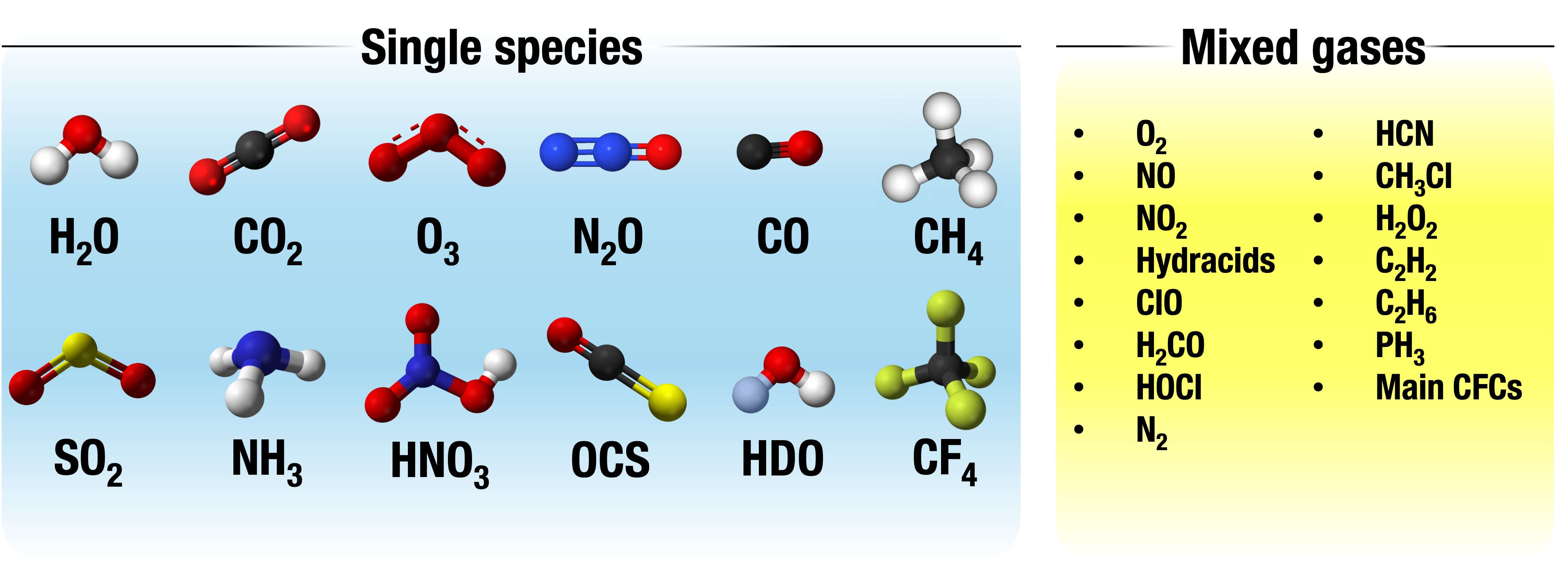
SIGMA includes coefficients to simulate 12 variable gas species, which are listed here below. The other atmospheric species are parametrized all together as "mixed gases" and include all species whose radiative impact in the TIR and FIR is small compared to the main species. Their concentration is fixed to the U.S. Standard atmosphere, yet their optical depth is correctly scaled with the input atmospheric temperature.

Input atmosphere  
The fact that the atmospheric layering is fixed in SIGMA implies that every calculation will be performed on this fixed layering. Nevertheless, the user has an extra degree of freedom in the specification of the input atmosphere, as the model can ingest values of pressure, temperature and abundances either on atmospheric levels, or on the set of 60 layers on which calculations are performed internally by the model.
In the first case, the user is free to specify parameters on any pressure grid. After interpolating those values on the 61 pressure levels embedded in SIGMA, the code will compute the average layer parameters assuming that each parameter obeys to hydrostatic equilibrium and that, in a given layer, each parameter \(Y\) varies linearly with the logarithm of pressure:

\(Y_{average} = \frac{\int_{P_l}^{P_u} Y(p) dp}{P_l-P_u} \)
\(Y(P) = Y_u + (Y_l - Y_u) \frac{\log(P)-\log(P_u)}{\log(P_l)-\log(P_u)} \)

\( \xrightarrow{\text{exact solution}} Y_{average} = Y_u + \frac{Y_l - Y_u}{(\log(P_l)-\log(P_u))(P_l-P_u)} [ P_l(\log(P_l)-1) - P_u(\log(P_u)-1) - \log(P_u)(P_l-P_u) ] \)

where \( Y_l\) and \( Y_u\) refers to the value of the quantity at the upper and lower boundaries of the considered layer, and the same convention applies to pressure \( P\). SIGMA assumes the same functional form for all parameters (including particle sizes). The possibility to input values at atmospheric levels instead of layers is very useful when using SIGMA solely for radiative transfer purposes. When used in retrievals, instead, it is highly recommended to use SIGMA specifying directly layers' values, because retrievals are typically finalized to find out the atmospheric parameters in terms of average value of each parameter in each layer.
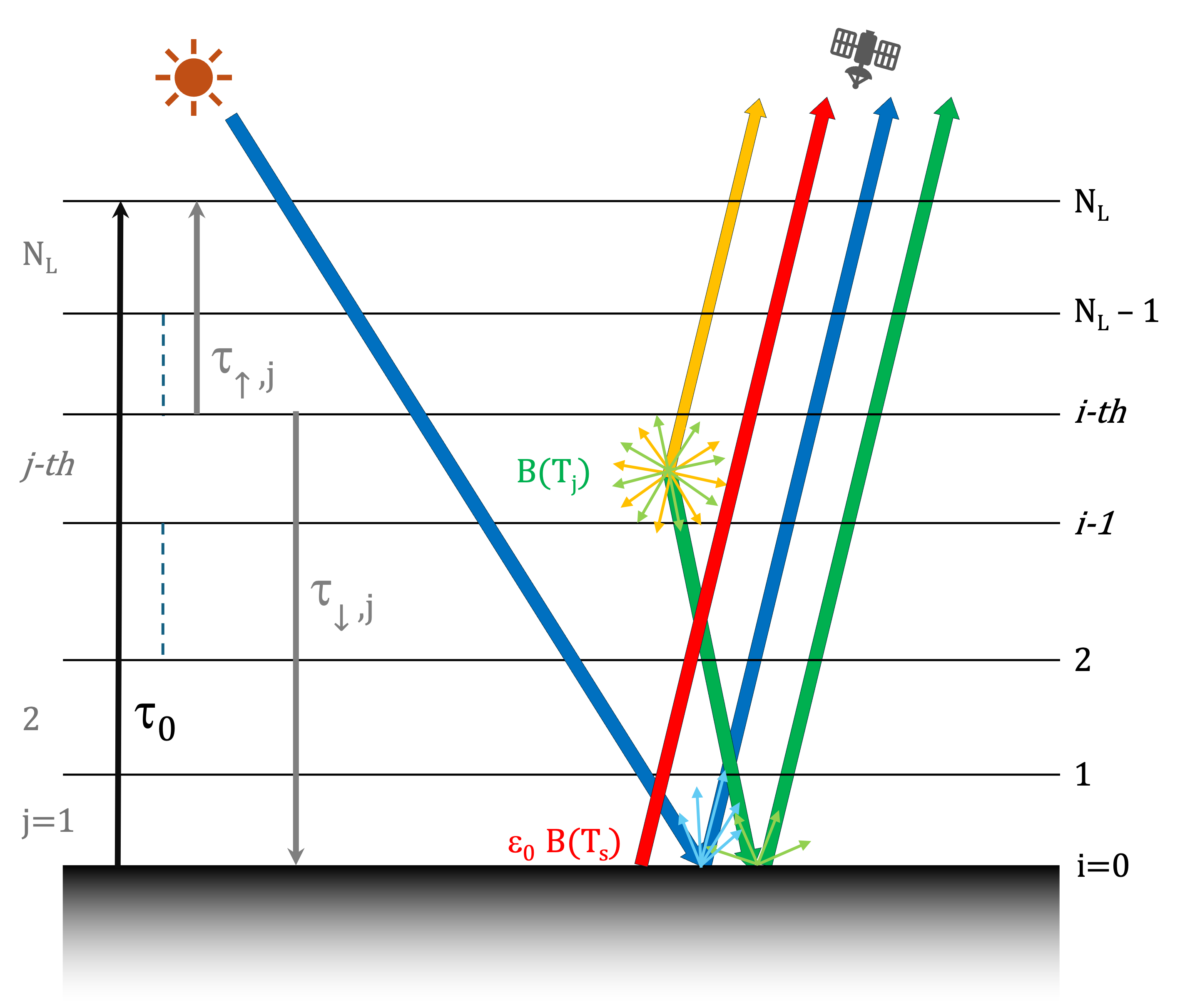
The Linear in T approximation  
When dealing with atmospheric layers that are very inhomogeneous, radiative transfer calculations can become more accurate by properly taking into account such inhomogeneities. One of the most critical situations is when there is a strong thermal gradient between the two boundaries and the layer is optically thick. Generally speaking, the integral expressing the atmosphere-emitted thermal radiation has an exact solution according to the "integral average theorem":

\( \int_{z_{j-1}}^{z_j} B(T) \frac{\partial τ}{\partial z} dz = B(T(z^*)) (τ_j - τ_{j-1}) \),   with   \( z_{j-1} \leq z^* \leq z_j \)

provided that \( \frac{\partial τ}{\partial z} \) does not change sign in the interval [\( z_{j-1}, z_{j}\)], which is generally true. Other schemes, such as LBLRTM, use a more crude approximation, usually called "Linear in τ" approximation (e.g., see Rodgers 2000). In this approximation, the integral above is calculated by considering that the Planck function B(T) is linear with the optical depth. The advantage of the formulation in SIGMA is the analytical solution of the above integral. In a practical case, when SIGMA is used for retrievals, \(T(z^*)\) is guessed equal to the layer's average temperature, and its final value is that which best fits the spectral 
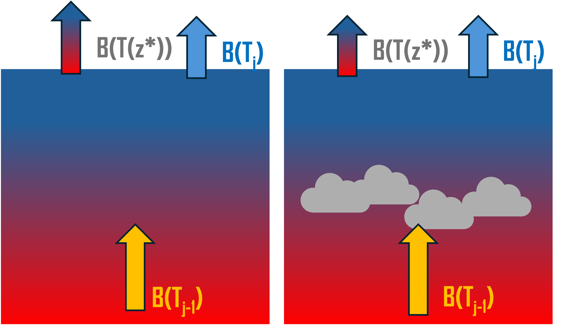
radiances. Yet, this can still be a too-crude approximation, especially for cloudy skies, which in the limit of overcast conditions, where the given j-th layer is opaque to the radiation coming from below, and the emitting temperature becomes that of the layer top. This is the case where SIGMA can be used activating what is named here the "Linear in T" approximation, which relies on the assumption that:

\( B(T(z^*)) = \frac{\int_{z_{j-1}}^{z_j} B(T) \frac{\partial τ}{\partial z} dz}{\int_{z_{j-1}}^{z_j} \frac{\partial τ}{\partial z} dz} \approx \frac{τ_j B(T_j) + τ_{j-1} B(T_{j-1})}{τ_j+τ_{j-1}} \)

which is the Planck function at the endpoints of the interval [\(z_{j-1}\),  \(z_{j}\)] weighted with the transmittance at the same endpoints. By considering the definition of transmittance, this can be cast in a more straightforward and immediate form:

\( B(T(z^*)) = \frac{B(T_j) + \exp(-χ_j) B(T_{j-1})}{1 + \exp(-χ_j)} \)

In this way, when the optical depth of the layer tends to zero, the equivalent blackbody radiation coming from the layer will be the average of the blackbodies of the two layer boundaries. Conversely, when the optical depth is very high, the equivalent blackbody radiation will be the one from the upper boundary. SIGMA allows for the use of this approximation at user's discretion, and it can be used either in clear or cloudy sky scenes.
Continuum absorption  
Besides line absorption, some gases in the Earth atmosphere yield an additional absorption contribution which is much more spectrally smooth than line absorption. For the most, this additional absorption can be explained by collisional effects, in which inelastic molecular collisions have a certain probability to activating specific absorption modes. Additionally, in the specific case of water vapor, the almost ubiquitous presence of spectral lines makes it difficult for line-by-line codes to account for the full line absorption, as such codes compute line shapes within ±25 cm-1 the line center. This underestimates the total line absorption especially in the core of roto-vibrational bands, and implies the need to introducing a non-parametric, additional continuum absorption term in the radiative transfer.
SIGMA includes all of these contributions, for the following specific collisional pairs: N2-N2, N2-O2 and O2-O2, which are the most common in Earth's atmosphere and are significant in the IR region. These absorptions are treated with the formalism of Collision-Induced Absorptions (CIAs) as seen in the HITRAN molecular spectroscopy database. The water vapor continuum is also treated with the very same formalism of the CIAs, despite its origin which is, overall, different. However, on the basis of the work done in Kofman & Villanueva (2021), it is easy to use the same mathematical formalism of the CIAs to treat water self and foreign continuum.
Calculations in SIGMA are performed with look-up tables of CIAs cross-sections at various temperatures, and with equivalent cross-sections for water self and foreign continua. This allows for calculations that are much more traceable than those in LBLRTM, and a code that is easy to maintain and update, instead of the rigid and cryptic LBLRTM contnm routine.


Clouds and Aerosols  

As previously mentioned, SIGMA includes advanced modules for calculating radiances in the presence of scattering layers, utilizing improved scaling methods that parameterize the optical depth of ice and liquid water clouds, as well as various aerosol species. These methodologies allow to avoid the direct calculation of the diffusion processes by scaling the absorption optical depth of the cloud. In this way, the effects induced by the multiple scattering are viewed in terms of absorption and emission processes. This allows the model to consider the radiative transfer problem in a Schwarzschild-like form, mitigating the computational burden of the solution.
SIGMA implements two scaling options: Chou's scaling solution and Tang's adjusted solution. The default one is the Chou approximation.
Chou's solution  
In the scheme proposed by Chou, the scattering contribution is accounted for by replacing the extinction optical depth of each atmospheric layer with an apparent optical depth, \(χ_{a}\).

\( \chi_{a} = \chi_{abs} + b \omega \chi_{ext} \)

Where \(χ_{abs}\) describes the true absorption by the layer itself, and the second term represents an effective absorption, reflecting the loss of radiation from the beam as a result of backscattering events. The information about multiple-scattering processes is codified in the backscattering parameter, \( b \). This parameter quantifies the average fraction of radiation that is scattered in the backward hemisphere and is formally derived by integrating the phase function of the cloud or aerosol over the backward directions.
Tang's solution  
Altought Chou's solutions can lead to accurate results for radiance simulations in the mid-infrared, different study (e.g. Martinazzo et al. 2021) have shown that when simulations of ice clouds in the FIR are considered, accurate results are obtained only in the case of optically thin clouds. To improve the accuracy of the scaling method proposed by Chou, an adjustment scheme is implemented following the work done by Tang et al. (2018). The main idea behind this adjustment scheme is to improve the approximation for the downward ambient radiance made by Chou when solving for the upward radiance. Specifically, the downward ambient radiation is computed as the Schwarzschild solution from the top-of-the-atmosphere to the surface, leading to a correction term of the form:

\( R_{j}^{Tang} = \frac{1}{2}\frac{\omega_j}{1-\omega_j(1-b_j)}\left[[R_j(-\mu)-B_j]\cdot [1-e^{-2\frac{(1-\omega_j(1-b_j))\chi_j}{\mu}}] \right] \)

\( R_{Tang} = \sum_j R_{j}^{Tang} \tau_{\uparrow,j} \)

Where \(R^{Tang}_{j}\) is the correction contribution from layer j and \(R_{Tang}\) is the total correction. Since this adjustment scheme was developed for flux calculations, its direct application to spectral radiance calculations, accounting for specific observation geometry, may introduce errors. To extend Tang's scheme to radiance calculations, we compute a correction coefficient \(k(\mu)\) that accounts for radiance anisotropy. The correction for the layer j becomes:

\( R_{j}^{Tang} = k_j(\mu)\frac{\omega_j}{1-\omega_j(1-b_j)}\left[[R_j(-\mu)-B_j]\cdot [1-e^{-2\frac{(1-\omega_j(1-b_j))\chi_j}{\mu}}] \right] \)

In the original work from Tang et al (2018), a correction term is proposed for fluxes computation \(k(\mu)=k=0.3\). SIGMA employs a set of \(k\) to account for different observational angles and particle habits. Given this correction, SIGMA will solve the radiative transfer problem in the form:

\[ \textcolor{black}{ R_{total}(σ) } = \textcolor{red}{ R_{surface}(σ) } + \textcolor{#c17106}{ R_{up}(σ) } + \textcolor{green}{ R_{down}(σ) } + \textcolor{blue}{ R_{☉}(σ) } +\textcolor{black}{ R_{Tang}(σ)} \]

Liquid water clouds  
Liquid water clouds are assumed as composed of a particle size distribution (PSD) of water spheres, whose single scattering single particle radiative properties are generated by using a Mie solution based algorithm. Water refractive indeces by Dowing and Williams (1975) are ingested for the computations. The single particle properties are then combined to generate single scattering radiative properties for the PSDs over the spectral interval of interest. PSDs of low-level stratiform clouds, as those modelled in this study, are commonly described by a lognormal distribution.
A table describing the water cloud properties contained in SIGMA is provided here:
Properties PSD type Effective Radii range Shape Parameter​ Tang adjustment​​
Liquid water cloud (Downing and Williams, 1975) Lognormal 1.5-30 \(\mu m\) \(\sigma = 0.1\) Yes
Ice water clouds  
Ice clouds are commonly assumed as PSDs of non-spherical ice crystals. In nature, multiple crystal shapes are observed within ice cloud layers depending on the cloud formation conditions, its evolution, and thermodynamic state. SIGMA implements crystal aggregates of eight hexagonal ice columns, whose single scattering single particle radiative properties are described by Yang et al. (2013). A commonly used PSD for ice clouds is the three parameters gamma distribution.
A table describing the ice cloud properties contained in SIGMA is provided here:
Properties PSD type Effective Radii range Shape Parameter​ Tang adjustment​​
Columnar Aggregates (Ping Yang, 2013)​ Gamma 4-100 \(\mu m\) \(\mu = 7\) Yes
Hexagonal plates (Ping Yang, 2013)​ Gamma 4-100 \(\mu m\) \(\mu = 7\) No
Hexagonal columns (Ping Yang, 2013)​ Gamma 4-100 \(\mu m\) \(\mu = 7\) No
Bullet rosettes (Ping Yang, 2013)​ Gamma 4-100 \(\mu m\) \(\mu = 7\) No
Mixed phases (Warren and Brandt, 2008)​​ Gamma 4-100 \(\mu m\) \(\mu = 7\) No
PSC type II (Ice) (Warren and Brandt, 2008) Lognormal 0.5-30 \(\mu m\) \(\sigma = 0.41\) No
Aerosols  
Globally, aerosols comprise a large variety of radiative proper ties due to variation in chemical composition, particle size distributions (often multimodal), and vertical concentration. Even if the most important impact on atmospheric radiances is at short wavelengths (0.3–4 \(\mu m)\) for some types of aerosols their effects at long wavelengths (4–100 \(\mu m)\) is not negligible and must be accounted for in radiative transfer computations.
A table describing the aerosol particles contained in SIGMA is provided here:
Properties PSD type Effective Radii range Shape Parameter​ Tang adjustment​​
Volcanic dust (HITRAN database)​ Lognormal 0.01-20 \(\mu m\) \(\sigma = 0.53\) No
Mineral transported (HITRAN database)​​ Lognormal 0.01-20 \(\mu m\) \(\sigma = 0.73\) No
Black carbon (HITRAN database)​​ Lognormal 0.01-20 \(\mu m\) \(\sigma = 0.69\) No


Surface Modeling  

SIGMA adopts the simplest approach to deal with surface properties. The model handles two different reflectance models, the specular and the Lambertian models. In the first case, given θobs the observation angle, surface is assumed to scatter radiation with the same angle in the same plane and opposite direction. In the case of Lambertian surface, radiation is scattered isotropically, such that the BRDF (Bi-directional Reflectance Distribution Function) is BRDF = r/π, with r the surface albedo (0 to 1).
While specular reflection in partticularly suitable for surfaces such as sea, ice sheets, or any other case in which there is a generally smooth surface, Lambertian reflection is of more general application, and adapts well to any common terrestrial surface and instruments with a Field of View large enough to encompass a wide variety of surfaces. To keep the scheme parametric also for emissivity, the computation of Lambertian albedo considers the so-called Elsasser approximation, in which an effective reflectance angle of 52.93 deg is assumed for the atmospheric-emitted reflected radiation.
In any case, SIGMA requires that the albedo is directly provided by the user in form of emissivity in the configuration, either as a spectrally variable emissivity or as a constant value across the spectral range of interest.
In case of satellite observations over bodies of water, the solar reflected radiation is treated differently than the thermal downwelling atmospheric radiation, as the latter one can be assumed isotropic, while the former is coming from a specific direction. To treat the solar component in this case, SIGMA implements a sunglint model, which computes the Fresnel reflectance of a body of water (based on water refractive index), and parametrizes the effects of marine surface roughness with a Cox-Munk parametrization as a function of wind speed.
The effect is prominent at wavelengths shorter than 5 μm, where the effect of solar radiation in satellite observations starts to dominate over the thermal emitted radiation from Earth.
Specular vs. Lambertian reflection
Cox-Munk reflectance examples


Instruments  

While it was originally built specifically to simulate radiances from hyperspectral IR sounders such as IASI, SIGMA has evolved and has been adapted to work with any instrument observing in the spectral interval 10-2800 cm-1, or having any/part of its spectral channels comprised in this interval. Other parametric codes (such as RTTOV) work in such a way that look-up tables for optical depths' calculations are heavily customized on the instrument to be simulated, allowing the possibility to use the code only with specific instruments. SIGMA works on a philosophy that, instead, is much closer to that of line-by-line codes: first, SIGMA simulates radiances, transmittances and jacobians at a resolution that is much higher than the observational one. These quantities are then convolved by the model a-posterior through a dedicated convolution routine. This approach allows to obtain accurate high resolution quantities, and the corresponding convolved ones, preserving efficiency, speed and accuracy simultaneously.
Given \(R(σ)\) a 1-D high-resolution quantity computed by SIGMA, and \(f_{inst}(σ-σ_i)\) the Instrument Spectral Response Function (ISRF) of the instrument's i-th spectral channel centred on \(σ_i\), the model computes the low-resolution, or instrument-like quantity \(r(σ_{i})\) at \(σ_i\) as follows:

\(r(σ_{i}) = \sum_{j=j_0-n}^{j_0+n} R(σ_j) f_{inst}(σ_j-σ_i)\)

with \(j_0\) the index of the high-resolution grid corresponding to the wavelength of the i-th spectral channel, and \(n\) the number of high-resolution points corresponding to the width of the ISRF (usually 6 standard deviations for a Gaussian ISRF).
The convolved radiances can be produced in two different modes:
  • an "instrument mode", which can be activated by specifying an instrument name in the configuration file. SIGMA has about 40 ISRF models available. If the specified instrument is one of the available ones, the code will produce low-resolution radiances, transmittances and jacobians using the corresponding ISRF. The spectral interval is also set accordingly.
  • a "custom mode", in which the user specifies the spectral interval of interest, the resolution, and the sampling, and the model convolves high resolution radiances, transmittances and jacobians with a Gaussian kernel of Full Width at Half Maximum equal to the resolution. The sampling defines, instead, the position of the spectral points in an equally spaced spectral grid from the lower to the upper wavenumber/wavelength defined by the user, and can be as fine as desired by the user.
In either case, according to the effective resolution of the instrument, radiative transfer calculations are performed using two look-up tables of optical depths, computed at resolutions of 0.01 cm-1 and 0.1 cm-1. If the requested resolution is coarser than 5 cm-1, SIGMA will use the look-up table at a resolution of 0.1 cm-1, otherwise it will use the look-up table at a resolution of 0.01 cm-1. In the first case, which is common among radiometers and imagers, calculations will be much faster while preserving accuracy at the instrument resolution with no noticeable bias.
SIGMA can also handle a variety of wavelength units (cm-1, μm, or nm), which are the most commonly used in the infrared domain, with the only constraint for the user to specifying the spectral interval, resolution and sampling in the same unit. Internally, SIGMA performs all its calculations in the native unit of cm-1 and with various optimization strategies.


Outputs  

SIGMA allows to calculate several output quantities handling a veriety of different units. The main capability of the code is to compute radiances, transmittances and especially analytical derivatives (Jacobians) of the radiance with respect to a set of atmospheric and surface parameters. The possibility to compute Jacobians analytically is granted by the polynomial treatment of optical depths both for gases and for aerosols, and by the linearity of the radiative transfer equation with respect to surface parameters.
Radiances and jacobians can be provided in units of wavelengths (μm or nm) or wavenumbers (cm-1), with the latter being the native unit in which calculations are internally performed in SIGMA. Additionally, the model is able to produce outputs in radiance units or equivalent brightness temperature, which is defined according to the Planck blackbody laws. The complete set of units and their conversion formulas is reported here below.


Wavelength unit Output unit Output Equation
wavenumbers [cm-1] Radiance [W m-2 sr-1 (cm-1)-1] Radiance \( \textcolor{green}{R'} = \textcolor{green}{R} \)
fundamental unit in SIGMA
Jacobian \( \textcolor{blue}{J'} = \textcolor{blue}{J} \)
fundamental unit in SIGMA
Brightness T [K] Radiance \( \textcolor{green}{R'} = \frac{PT}{\log(1+PF/\textcolor{green}{R})} \)
Jacobian \( \textcolor{blue}{J'} = \frac{PF \cdot PT}{\log^2(1+PF/\textcolor{green}{R})} \frac{\textcolor{blue}{J}}{\textcolor{green}{R}(\textcolor{green}{R}+PF)} \)
\( PT=C2 \cdot σ, PF=C1 \cdot σ^3 \), with \(C1=1.19104 \cdot 10^{-8}, C2=1.43877, σ\) in cm-1
microns [μm] Radiance [W m-2 sr-1 μm-1] Radiance \( \textcolor{green}{R'} = \textcolor{green}{R} \cdot σ^2 \cdot 10^{-4} \)
Jacobian \( \textcolor{blue}{J'} = \textcolor{blue}{J} \cdot σ^2 \cdot 10^{-4} \)
Brightness T [K] Radiance \( \textcolor{green}{R'} = \frac{PT}{\log(1+PF/\textcolor{green}{R})} \)
Jacobian \( \textcolor{blue}{J'} = \frac{PF \cdot PT}{\log^2(1+PF/\textcolor{green}{R})} \frac{\textcolor{blue}{J}}{\textcolor{green}{R}(\textcolor{green}{R}+PF)} \)
\( PT=\frac{HCK}{λ}, PF=\frac{HCJ}{λ^5} \), with \(HCK=1.43877 \cdot 10^4, HCJ = 1.19104 \cdot 10^8, λ\) in μm
nanometers [nm] Radiance [W m-2 sr-1 nm-1] Radiance \( \textcolor{green}{R'} = \textcolor{green}{R} \cdot σ^2 \cdot 10^{-7} \)
Jacobian \( \textcolor{blue}{J'} = \textcolor{blue}{J} \cdot σ^2 \cdot 10^{-7} \)
Brightness T [K] Radiance \( \textcolor{green}{R'} = \frac{PT}{\log(1+PF/\textcolor{green}{R})} \)
Jacobian \( \textcolor{blue}{J'} = \frac{PF \cdot PT}{\log^2(1+PF/\textcolor{green}{R})} \frac{\textcolor{blue}{J}}{\textcolor{green}{R}(\textcolor{green}{R}+PF)} \)
\( PT=\frac{HCK}{λ}, PF=\frac{HCJ}{λ^5} \), with \(HCK=1.43877 \cdot 10^4, HCJ = 1.19104 \cdot 10^8, λ\) in nm