| "GEOMETRY-TYPE" | "-" | "Observing geometry of the model. It can be Nadir, Zenith or looking to the Sun from the surface. " |
| "GEOMETRY-TIME" | "-" | "Date and time of the observation in UT. Format: YYYY\/MM\/DD hh:mm. " |
| "GEOMETRY-LATITUDE" | "N deg" | "Northern latitude of the target. " |
| "GEOMETRY-LONGITUDE" | "E deg" | "Eastern longitude of the target. " |
| "GEOMETRY-VIEW-ANGLE" | "deg" | "Angle between the normal to the surface and the observing direction. " |
| "GEOMETRY-SUN-ANGLE" | "deg" | "Angle between the normal to the surface and the direction to the Sun. " |
| "GEOMETRY-VIEW-AZIMUTH" | "deg" | "Angle between the local North and the observing direction. " |
| "GEOMETRY-SUN-AZIMUTH" | "deg" | "Angle between the local North and the Sun-target direction at the surface. " |
| "GEOMETRY-SUN-DIST" | "AU" | "Distance between the Earth and the Sun in Astronomical Units. " |
| "ATMOSPHERE-PRESS-OBSERVER" | "mbar" | "Atmospheric pressure at which the observer is located. It can be 0.005 to 1030 mbar or equivalent unit. " |
| "ATMOSPHERE-PRESS-TARGET" | "mbar" | "Atmospheric pressure at which the target is observed. It can be 0.005 to 1030 mbar or equivalent unit. " |
| "ATMOSPHERE-PRESS-UNIT" | "mbar" | "Unit for the specified atmospheric pressure; choices are mbar, pascal, atm or bar. " |
| "ATMOSPHERE-SPECIES" | "-" | "List of the species that are present in the atmosphere. They must be among those for which a profile is provided. Options are: H2O,CO2,O3,N2O,CO,CH4,SO2,HNO3,NH3,OCS,HDO,CF4. " |
| "ATMOSPHERE-ABUNDANCES" | "-" | "Abundance of the species, which can be specified in several units; scf is for scaler of the provided profile. " |
| "ATMOSPHERE-UNITS" | "-" | "Units of the abundances. Options: scf, ppmv, ppbv, pptv, pct; anything different from scf will replace the provided profile with a constant one of the specified value. " |
| "ATMOSPHERE-CLOUDS" | "-" | "Types of clouds and aerosols that are in the atmosphere. Their profile must be in the section. " |
| "ATMOSPHERE-CLOUD-ABUN" | "-" | "Abundance of the types of clouds and aerosols present in the atmosphere. Their profile must be in the section. " |
| "ATMOSPHERE-CLOUD-UNIT" | "-" | "Unit of the abundance of the types of clouds present in the atmosphere. Their profile must be in the section. " |
| "ATMOSPHERE-CLOUD-FRAC" | "-" | "Fraction of the FOV covered by clouds and\/or aerosols. It is assumed common for both water and ice. " |
| "ATMOSPHERE-PROFILES" | "-" | "Species for which a profile is provided. H2O must be in g\/kg, the others in ppmv, aerosol sizes in um. " |
| "ATMOSPHERE-NLAYERS" | "-" | "Number of atmospheric layers. It has to be the same as the number of layers effectively in the config file, which go from the surface pressure to the top of the atmosphere. Admissibile values go from 1 to 140. " |
| "ATMOSPHERE" | "-" | "User-supplied atmosphere. It is integrated in the config file through the tags and <\/ATMOSPHERE>. It includes pressure, temperature and the species indicated in the tag " |
| "ATMOSPHERE-TANG" | "-" | "Flag to apply the Tang correction to cloudy spectra. Works only for upwelling radiances. " |
| "ATMOSPHERE-LINEART" | "-" | "Switch to apply the linear-in-T approximation to radiance calculations. Useful for very inhomogeneous layers. " |
| "ATMOSPHERE-LEVELS" | "-" | "Switch to specify whether the user atmosphere contains values on boundaries (Y) or averaged on layers (N). " |
| "SURFACE-TEMPERATURE" | "K" | "Skin temperature of the surface. " |
| "SURFACE-EMISSIVITY" | "-" | "Emissivity of the surface. It is a single value that is applied to the whole spectral range. If an emissivity spectrum is present, this entry is ignored. " |
| "SURFACE-TYPE" | "-" | "Surface type, indicating whether the surface is a Lambertian reflector or a specular one. " |
| "SURFACE-WIND" | "m\/s" | "Wind speed at the surface. It is needed to model sunglint with a Cox-Munk model on the sea. Otherwise, it is ignored. " |
| "INSTRUMENT-WAVE1" | "-" | "Initial wavelength or frequency of the calculation. " |
| "INSTRUMENT-WAVE2" | "-" | "Final wavelength or frequency of the calculation. " |
| "INSTRUMENT-RESOLUTION" | "-" | "Spectral resolution expressed as FWHM of the gaussian filter applied to the data. It must be given in the same unit as the wavelengths. If it is a radiometer among those available, this number is ignored. " |
| "INSTRUMENT-SAMPLING" | "-" | "Spectral sampling. It must be given in the same unit as the wavelengths. If it is not specified, it is put equal to the resolution. " |
| "INSTRUMENT-WAVE-UNIT" | "-" | "Unit in which the wavelength or frequency is expressed. Options are cm-1,um,nm. " |
| "INSTRUMENT-NAME" | "-" | "Choice of instruments to load presets and spectral response functions from. " |
| "INSTRUMENT-OUTPUT" | "-" | "Output terms wanted from the radiance calculations. " |
| "INSTRUMENT-OUTPUT-UNIT" | "-" | "Unit of the output radiance and Jacobians. It can be radiance units (RU) or brightness temperature (BT). " |
| "RETRIEVAL-VARIABLES" | "-" | "Jacobians wanted from the radiative transfer calculations. They can be only variables included in the radiative transfer profiles. " |
| "SPEC" | "-" | "User-supplied emissivity. It is integrated in the config file through the tags and <\/SPEC> including wavenumbers and values" |
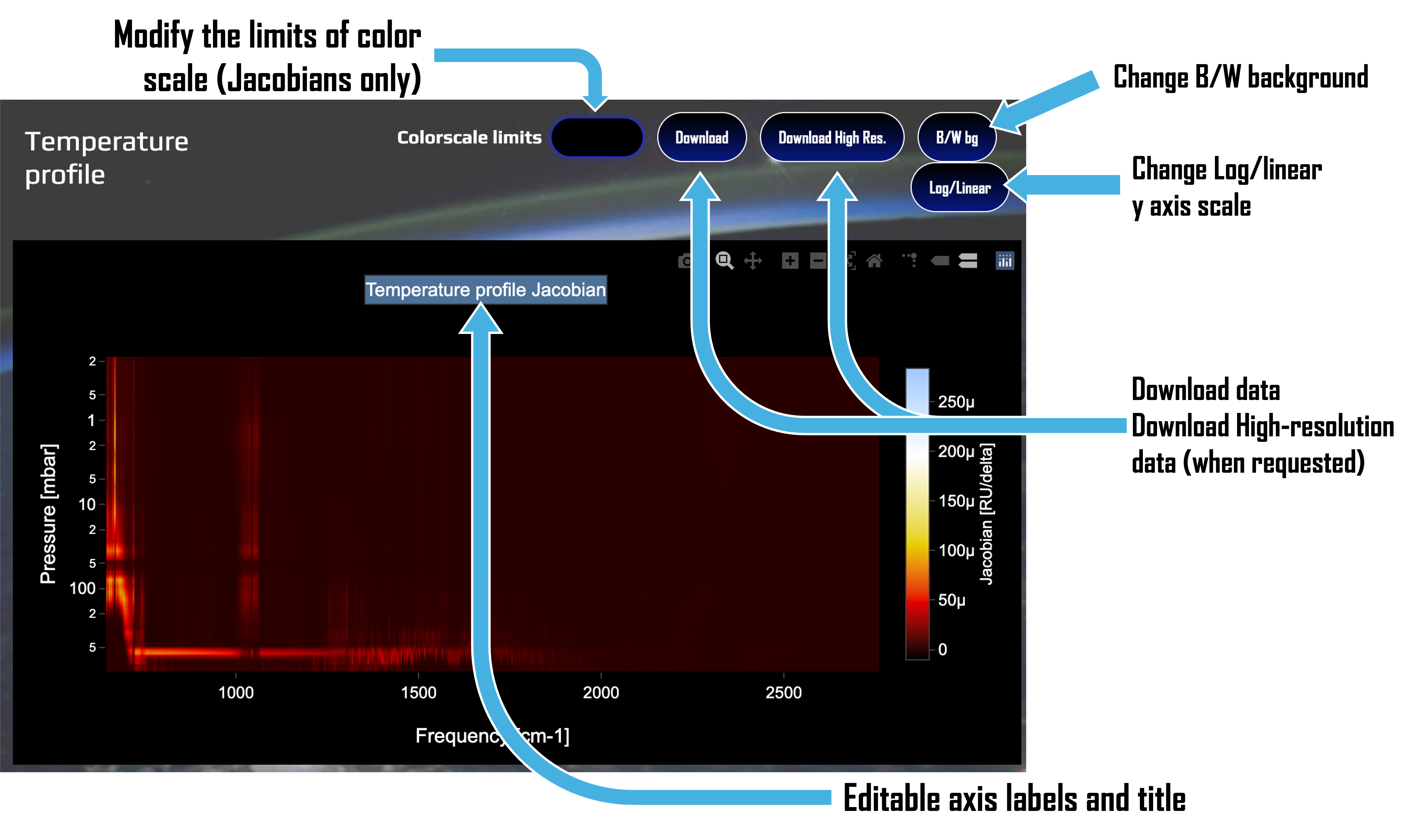
 The GUI also allow to easily work on plots. Depending on the choice of a custom instrument or a specific one with low resolution, radiances
are plotted either as a simple spectrum (wavelength vs. signal) or as a point-spectrum with the spectral response functions of each
channel. Jacobians, instead, are plotted as a 2D colormap (wavelength vs. pressure and the color indicating the value), and can be edited
to the choice of the user, as detailed below here.
The GUI also allow to easily work on plots. Depending on the choice of a custom instrument or a specific one with low resolution, radiances
are plotted either as a simple spectrum (wavelength vs. signal) or as a point-spectrum with the spectral response functions of each
channel. Jacobians, instead, are plotted as a 2D colormap (wavelength vs. pressure and the color indicating the value), and can be edited
to the choice of the user, as detailed below here.